axis · graph · graphmode · plot · plotx · ploty · plt · regraph · setcolor · settext

Obsolete Plotting

Warning

The functions on this page should be considered obsolete and avoided in new code; use Graph or regular Python (matplotlib, plotnine, plotly, …) or MATLAB graphics instead.

graphmode()

Python

obsolete. Use Graph instead.

Syntax:

n.graphmode(1)

Executes the list of setup statements. This is also done on the first call to n.graph(t) after a new setup statement is added to the list.

n.graphmode(-1)

Flushes the stored plots. Subsequent calls to n.graph(t) will start new lines. Should be executed just before a n.plt(-1) to ensure the entire lines are plotted.

n.graphmode(2)

Flushes the stored plots. Subsequent calls to n.graph(t) will continue the lines. Graphs are normally flushed every 50 points.

HOC

obsolete. see graph(). Use Graph.

---

graph()

Python

obsolete; use Graph instead

Syntax:

n.graph()

n.graph(expression, setup)

n.graph(t)

n.graphmode(mode)

Description:

The graph() function solves the problem of obtaining multiple line plots during a single run. During calls to n.graph(t), specified variables are stored and plotted using scales determined by calls to axis().

Options:

n.graph()

erases the old list and starts a new (empty) list of plot expressions and setup statements.

n.graph(s1, s2)

Adds a new plot specification to the graph list. s1 must be a string which contains a HOC expression, usually a variable. e.g "y". s2 is a string which contains any number of HOC statements used to initialize axes. etc. E.G "axis(0,5,1,-1,1,2) axis()".

n.graph(t)

The current value of each expression in the graph list is saved along with the abscissa value, t. The line plots are flushed every 50 points.

Example:

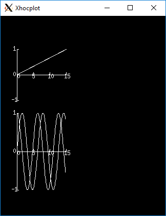
from neuron import n, gui
import numpy as np

# define a HOC variable x
n('x = 0')


def p(): # plot ramp
    n.axis(100, 300, 450, 200)
    n.axis(0, 15, 3, -1, 1, 2)
    n.axis()
    n.plot(1)
    for n.x in np.arange(0, 15, 0.1):
        # using n.x instead of x is essential to allow the sin and
        # cos graphs to update
        n.plot(n.x, n.x / 15.)    # ramp
        n.graph(n.x)  # plots graph list if any
    n.graph(-1)  # flush remaining part of graphs, if any
    n.plt(-1)


p()    # plots the ramp alone

n.graph()
# x here refers to the variable known to Python as n.x
n.graph("sin(x)","axis(100, 300, 100, 300) axis()")
n.graph("cos(x)", "")  # same axes as previous call to graph

p()    # plots the sin and cos along with the ramp

Diagnostics:

The strings are parsed when n.graph(s1, s2) is executed. The strings are executed on calls to n.graph(t).

The best method for complicated plots is to make the setup string a simple call to a user defined procedure. This procedure can setup the axes, write the labels, etc. Newlines and strings within strings are possible by quoting with the \ character but generally are too confusing to be practical.

Local variables in graph strings make no sense.

Note

All expressions for initialization and for plotting must be specified as HOC expressions not as Python callables. These functions are maintained solely to maintain backward compatability, so this limitation is likely to never be lifted. New code should use Graph instead, which does not have this limitation.

Note

On some modern systems, the graph window may have to be interacted with (e.g. resized) before the first graph will appear.

See also

plot(), Graph

HOC

Name:

graph — multiple line plots

Syntax:

graph()

graph(expression, setup)

graph(t)

graphmode(mode)

Description:

Graph() solves the problem of obtaining multiple line plots during a single run. During calls to graph(t), specified variables are stored and plotted using scales determined by calls to axis().

Options:

graph()

erases the old list and starts a new (empty) list of plot expressions and setup statements.

graph(s1, s2)

Adds a new plot specification to the graph list. s1 must be string which contains an expression, usually a variable. e.g “y”. s2 is a string which contains any number of statements used to initialize axes. etc. E.G “axis(0,5,1,-1,1,2) axis()”.

graph(t)

The current value of each expression in the graph list is saved along with the abscissa value, t. The line plots are flushed every 50 points.

graphmode(1)

Executes the list of setup statements. This is also done on the first call to graph(t) after a new setup statement is added to the list.

graphmode(-1)

Flushes the stored plots. Subsequent calls to graph(t) will start new lines. Should be executed just before a plt(-1) to ensure the entire lines are plotted.

graphmode(2)

Flushes the stored plots. Subsequent calls to graph(t) will continue the lines. Graphs are normally flushed every 50 points.

Example:

proc p() { /* plot ramp */
   axis(100,300,450,200)
   axis(0,15,3,-1,1,2)
   axis()
   plot(1)
   for (x=0; x<15; x=x+.1) {
      plot(x, x/15) /* ramp */
      graph(x) /* plots graph list if any */
   }
   graph(-1) /* flush remaining part of graphs, if any */
   plt(-1)
}


p()    /*plots the ramp alone*/


graph()
graph("sin(x)","axis(100,300,100,300) axis()")
graph("cos(x)","")  /* same axes as previous call to graph */


p()    /* plots the sin and cos along with the ramp */

Diagnostics:

The strings are parsed when graph(s1, s2) is executed. The strings are executed on calls to graph(t).

The best method for complicated plots is to make the setup string a simple call to a user defined procedure. This procedure can setup the axes, write the labels, etc. Newlines and strings within strings are possible by quoting with the ‘verb++’ character but generally are too confusing to be practical.

Local variables in graph strings make no sense.

See also

plot()

---

axis()

Python

Syntax:

n.axis()

n.axis(clip)

n.axis(xorg, xsize, yorg, ysize)

n.axis(xstart, xstop, nticx, ystart, ystop, nticy)

Options:

n.axis()

draw axes with label values. Closes plot device.

n.axis(clip)

points are not plotted if they are a factor clip off the axis scale. Default is no clipping. Set clip to 1 to not plot out of axis region. A value of 1.1 allows plotting slightly outside the axis boundaries.

n.axis(xorg, xsize, yorg, ysize)

Size and location of the plot region. (Use the n.plt() absolute coordinates.)

n.axis(xstart, xstop, nticx, ystart, ystop, nticy)

Determines relative scale and origin.

See also

plot()

HOC

See plot()

---

plotx()

---

ploty()

---

regraph()

Python

See graph()

HOC

See graph()

---

plot()

Python

Syntax:

n.plot(mode)

inrange = n.plot(x, y)

Description:

n.plot() plots relative to the origin and scale defined by calls to axis(). The default x and y axes have relative units of 0 to 1 with the plot located in a 5x3.5 inch area.

Options:

n.plot()

print parameter usage help lines.

n.plot(0)

subsequent calls will plot points.

n.plot(1)

next call will be a move, subsequent call will draw lines.

n.plot(x, y)

plots a point (or vector) relative to the axis scale. Return value is 0 if the point is clipped (out of range).

n.plot(mode, x, y)

Like plt() but with scale and origin given by axis().

Example:

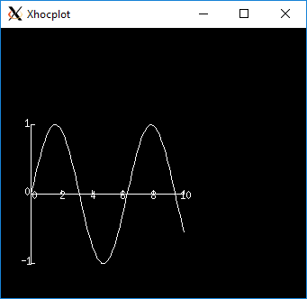
from neuron import n, gui
import numpy as np

# plot the sin function from 0 to 10 radians
n.axis(0, 10, 5, -1, 1, 2) # setup scale
n.plot(1)
for x in np.linspace(0, 10, 100):
    n.plot(x, np.sin(x))  # plot the function

n.axis()

See also

plt(), setcolor(), axis()

HOC

Name: plot, axis - plot relative to scale given by axes

Syntax:

axis(args)

plot(mode)

inrange = plot(x,y)

Description:

Plot() plots relative to the origin and scale defined by calls to axis. The default x and y axes have relative units of 0 to 1 with the plot located in a 5x3.5 inch area.

Options:

plot()

print parameter usage help lines.

plot(0)

subsequent calls will plot points.

plot(1)

next call will be a move, subsequent call will draw lines.

plot(x, y)

plots a point (or vector) relative to the axis scale. Return value is 0 if the point is clipped (out of range).

plot(mode, x, y)

Like plt() but with scale and origin given by axis().

axis()

draw axes with label values. Closes plot device.

axis(clip)

points are not plotted if they are a factor clip off the axis scale. Default is no clipping. Set clip to 1 to not plot out of axis region. A value of 1.1 allows plotting slightly outside the axis boundaries.

axis(xorg, xsize, yorg, ysize)

Size and location of the plot region. (Use the plt() absolute coordinates.)

axis(xstart, xstop, nticx, ystart, ystop, nticy)

Determines relative scale and origin.

Specification of the precision of axis tic labels is available by recompiling hoc/SRC/plot.c with #define Jaslove 1+. With this definition, the number of tics specified in the 3rd and 6th arguments of axis() should be of the form m.n. m is the number of tic marks, and n is the number of digits after the decimal point which are printed. This contribution was made by Stewart Jaslove.

Example:

proc plotsin() { /* plot the sin function from 0 to 10 radians */
axis(0, 10, 5, -1, 1, 2) /* setup scale */
plot(1)
for (x=0; x<=10; x=x+.1) {
    plot(x, sin(x)) /* plot the function */
}
axis() /* draw the axes */
}

See also

plt(), setcolor(), axis()

---

setcolor()

Python

obsolete.

Syntax:

n.setcolor(colorval)

Description:

n.setcolor() sets the color (or pen number for HP plotter) used for plt().

Argument to n.setcolor() produces the following screen colors with an EGA adapter (left), X11 graphics (right):

Color Mapping Table

Code	HP Plotter Color	Alternate Color
0	black (pen 1)	black
1	blue	white
2	green	yellow
3	cyan	red
4	red	green
5	magenta	blue
6	brown	violet
7	light gray (pen 1)	cyan
…	…	…
15	white	green

HOC

obsolete. See plt().

---

settext()

Python

obsolete. See plt().

HOC

obsolete. See plt().

---

plt()

Python

Syntax:

n.plt(mode)

n.plt(mode, x, y)

Description:

n.plt() plots points, lines, and text using the Tektronix 4010 standard. Absolute coordinates of the lower left corner and upper right corner of the plot region are (0,0) and (1000, 780) respectively.

TURBO-C graphics drivers for VGA, EGA, CGA, and Hercules are automatically selected when the first plotting command is executed. An HP7475 compatible plotter may be connected to COM1:.

Options:

n.plt(-1)

Place cursor in home position.

n.plt(-2)

Subsequent text printed starting at current coordinate position.

n.plt(-3)

Erase screen, cursor in home position.

n.plt(-5)

Open HP plotter on PC; the plotter will stay open until another n.plt(-5) is executed.

n.plt(0, x, y)

Plot point.

n.plt(1, x, y)

Move to point without plotting.

n.plt(2, x, y)

Draw vector from former position to new position given by (x, y). (mode can be any number >= 2)

Several extra options are available for X11 graphics.

n.plt(-4, x, y)

Erases area defined by previous plot position and the point, (x, y).

n.plt(-5)

Fast mode. By default, the X11 server is flushed on every plot command so one can see the plot as it develops. Fast mode caches plot commands and only flushes on plt(-1) and setcolor(). Fast mode is three times faster than the default mode. It is most useful when plotting is the rate limiting step of the simulation.

n.plt(-6)

X11 server flushed on every plot call.

When the graphic window is resized, NEURON is notified after the next erase command.

Example:

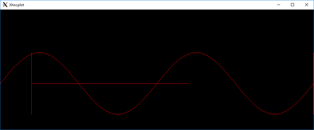
from neuron import n, gui
import math

n.setcolor(3)      # color 3 is red for X11; to use with EGA, change to 4
n.plt(1, 100, 500)
n.plt(2, 100, 100) # y-axis
n.plt(1, 100, 300)
n.plt(2, 600, 300) # x-axis (NOTE: does not correspond to origin of sine wave)
n.plt(1, 200, 550)
n.plt(-2)
for i in range(1001):
    n.plt(i + 1, i * 5, 300 + 200 * math.sin(2 * math.pi * i / 100.))

n.plt(-1) # close plot

See also

plot(), axis(), lw(), setcolor(), Graph

Warning

EGA adaptor used extensively but CGA and Hercules used hardly at all.

When the X11 graphic window is killed, NEURON exits without asking about unsaved edit buffers.

HOC

Name: plt, setcolor- low level plot functions

Syntax:

plt(mode)

plt(mode, x, y)

setcolor(colorval)

Description:

Plt() plots points, lines, and text using the Tektronix 4010 standard. Absolute coordinates of the lower left corner and upper right corner of the plot region are (0,0) and (1000, 780) respectively. Setcolor() sets the color (or pen number for HP plotter)

TURBO-C graphics drivers for VGA, EGA, CGA, and Hercules are automatically selected when the first plotting command is executed. An HP7475 compatible plotter may be connected to COM1:.

Options:

plt(-1)

Place cursor in home position.

plt(-2)

Subsequent text printed starting at current coordinate position.

plt(-3)

Erase screen, cursor in home position.

plt(-5)

Open HP plotter on PC.

setcolor()

The plotter will stay open till another plt(-5) is executed.

plt(0, x, y)

Plot point.

plt(1, x, y)

Move to point without plotting.

plt(2, x, y)

Draw vector from former position to new position given by (x,y). (mode can be any number >= 2)

Several extra options are available for X11 graphics.

plt(-4, x, y)

Erases area defined by previous plot position and the point, (x, y).

plt(-5)

Fast mode. By default, the X11 server is flushed on every plot command so one can see the plot as it develops. Fast mode caches plot commands and only flushes on plt(-1) and setcolor(). Fast mode is three times faster than the default mode. It is most useful when plotting is the rate limiting step of the simulation.

plt(-6)

X11 server flushed on every plot call.

When the graphic window is resized, hoc is notified after the next erase command.

Argument to setcolor() produces the following screen colors with an EGA adapter, X11 graphics:

0      black  (pen 1 on HP plotter)         black
1      blue                                 white
2      green                                yellow
3      cyan                                 red
4      red                                  green
5      magenta                              blue
6      brown                                violet
7      light gray  (pen 1 on HP plotter)    cyan
...
15     white                                green

Example:

proc plotsin() { /* This procedure plots the sin function in red.*/
setcolor(4)
plt(1, 100, 500)  plt(2, 100, 100) /* y-axis*/
plt(1, 100, 300)  plt(2, 600, 300) /* x-axis*/
plt(1, 200, 550)
plt(-2)  print "SIN(x) from 0 to 2*PI" /* label*/
for(i=0; i<=100;i=i+1){
    plt(i+1, i*500/100, 300 + 200*sin(2*PI*i/100))
}
plt(-1) /* close plot */
}

See also

plot(), axis(), lw()

Warning

EGA adaptor used extensively but CGA and Hercules used hardly at all.

When the X11 graphic window is killed, hoc exits without asking about unsaved edit buffers.